
Geotechnical engineering libraryContact
 benesch
Railroad Geotechnical Services Manual | Primary Source: USACE EM 1110-1-1804 All equations and parameters expressed in English (Imperial) units throughout.
Apps on dirtbert.com that support this chapter. Each one runs in a web browser on a desktop or a phone, with nothing to install. How to use the apps (I.3). Tools marked TOOLS open in the Geotechnical Analysis Suite (Benesch sign-in); the orange card below lists each one by section.
NANCY pages ask you to accept the Use and Disclaimers once in each browser. MINA is a monitoring aid and is not for operational dispatch decisions.
Calculators and workbook tools from the Benesch Geotechnical Analysis Suite that support this chapter: 1 interactive calculator and 3 workbook guides. Each one is also placed inside the section it supports, in an orange tools strip.
| SS | Residual & Fully Softened Strength CorrelationsUsed in 13.6 Residual Strength and Progressive Failure | Calculator ▸ | Guide |
| SS | Slope Stability — Effective StressUsed in 13.3 Limit Equilibrium Methods | guide only | Guide |
| SS | Slope Stability — Total StressUsed in 13.3 Limit Equilibrium Methods | guide only | Guide |
| SS | Staged Slope Stability — Pore PressureUsed in 13.3 Limit Equilibrium Methods | guide only | Guide |
Tools open on dirtbert.com and need the Benesch sign-in. Drafts pending Benesch final review, not for use in design.
General topic illustrations from Benesch's shared geotechnical graphics library, related to this chapter's subject matter — not the numbered figures called out in the text above. Click any image to view it full size.
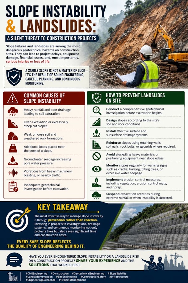
Slope stability governs the design of railroad embankments, cut slopes, and side-hill fills across all nine railroad client systems. An embankment failure — whether a rotational slide in soft foundation clay, a translational wedge along a shale bedding plane, or a surficial slump after heavy rainfall — can result in track loss, derailment, emergency speed restriction, and weeks of service disruption. This chapter develops the complete slope stability analysis framework: the Bishop Simplified method for circular failure surfaces, the Janbu Generalized method for non-circular surfaces, pseudo-static seismic analysis, tension crack depth, progressive failure in strain-softening clays, and cut slope design in rock. Minimum factors of safety follow USACE EM 1110-2-1902 as the primary criterion, supplemented by client-specific requirements from CSXT ES, NSR ESM, BNSF EI, UPRR EIM, CPKC TS, Amtrak ES, G&W EB, CN ES, and AREMA MRE Chapter 8. Three worked examples address an NSR Appalachian embankment over residual clay, a BNSF staged construction embankment over soft foundation soil, and a CPKC prairie cut slope in glacial till. A full slope stability analysis checklist, representative design tables, and five practice questions with complete answers are provided.
The correlations below are used or referenced in this chapter. Each is a statistical fit to a particular data set, so a value from one is an estimate: it applies only within the materials and ranges stated, carries the scatter of the original data, and must be confirmed by site-specific testing or calibration before it is relied on for design.
When an equation is used, note it with the result: give the equation ID and source, state that the soil or rock is within its range of applicability, mark the value as correlated (not tested), and record the limitation that governs. The Empirical Equations & Correlations reference has every entry with its full references.
Variables. PI = plasticity index (%)
Use. Soft clays, embankment stability on soft ground; based on back-analyzed failures. Typical PI 5–100%.
Limitations. Not applicable to fissured, varved, or organic clays without local calibration. Scatter about ±25%.
Source. Azzouz et al. 1983 (fit to Bjerrum 1972) · In this chapter: 13.1 · Full entry and references
Variables. PI (%)
Use. Normally consolidated clays (field vane basis).
Limitations. Field vane values; apply Bjerrum correction (IS-25) for stability. Not for OC clays.
Source. Skempton 1957 · Full entry and references
Variables. OCR = σ'p/σ'v0
Use. Mechanically overconsolidated, homogeneous clays; DSS loading (averaged mode).
Limitations. S and m vary with mode of shear, plasticity, and aging; determine from lab CK0U tests on project soils where possible.
Source. Ladd 1991; Mesri 1975 · Full entry and references
Variables. PI (%)
Use. Normally consolidated, inorganic clays; peak effective-stress φ'.
Limitations. Standard deviation about ±3°. Not residual or fully softened strength; for slope reactivation use residual/fully-softened correlations (e.g., Stark & Eid charts).
Source. Kulhawy & Mayne 1990 (data of Bjerrum & Simons 1960) · Full entry and references
Variables. f1 varies with plasticity index
Use. Insensitive, overconsolidated clays and weak rocks (U.K. data); PI ≈ 15–65%.
Limitations. Very large scatter; not reliable in soft or sensitive clays where N is very low. Use CPT, vane, or lab tests for design Su.
Source. Stroud 1974 · Full entry and references
Variables. Nkt = empirical cone factor, typically 10–20 (average ≈ 14); decreases with increasing Bq
Use. Fine-grained soils penetrated undrained (Ic > ~2.6).
Limitations. Nkt depends on reference test (vane, CIUC, DSS) and plasticity; calibrate locally. Use Nkt toward upper end for conservative Su.
Source. Lunne et al. 1997 · Full entry and references
Variables. RMRb = basic RMR (no orientation adjustment); F1 parallelism of joint/slope strike; F2 joint dip (planar); F3 joint-to-slope dip relation; F4 excavation method (+15 natural to −8 deficient blasting)
Use. Rock slopes; planar and toppling modes (wedge by pairwise check).
Limitations. Continuous-function forms (Tomás et al. 2007) reduce step artifacts. Does not replace kinematic and limit-equilibrium analysis.
Source. Romana 1985 · Full entry and references
Variables. σci = intact UCS; mi = intact rock constant; D = disturbance factor (0 undisturbed – 1 heavily blasted)
Use. Isotropic, heavily jointed rock masses (4+ joint sets) or intact rock.
Limitations. Not for rock masses where failure is controlled by one or two discrete discontinuity sets; use structural (kinematic) analysis there. D strongly affects results in slopes.
Source. Hoek et al. 2002 · Full entry and references
Variables. JRC = joint roughness coefficient (0–20); JCS = joint wall compressive strength; φb = basic friction angle; r, R = Schmidt rebound on weathered and fresh surfaces
Use. Unfilled rock joints at low to moderate normal stress.
Limitations. Limit arctan term to ≤ 70°. Scale effects reduce JRC and JCS at field scale (Bandis et al. 1981). Not for infilled joints.
Source. Barton & Choubey 1977 · Full entry and references
Slope failures impose direct costs on railroad operations through emergency repair, traffic rerouting, crane mobilization, and environmental spill response. They impose indirect costs through locomotive speed restrictions, customer delivery failures, and regulatory scrutiny. The Federal Railroad Administration does not prescribe slope stability factors of safety directly, but 49 CFR Part 213 mandates that track geometry be maintained within class tolerances — a failed or deforming slope that moves the track out of tolerance triggers an immediate slow order or line closure under FRA authority.
Each railroad client's approach to slope stability risk reflects its operational philosophy and geographic exposure:
Reference graphics
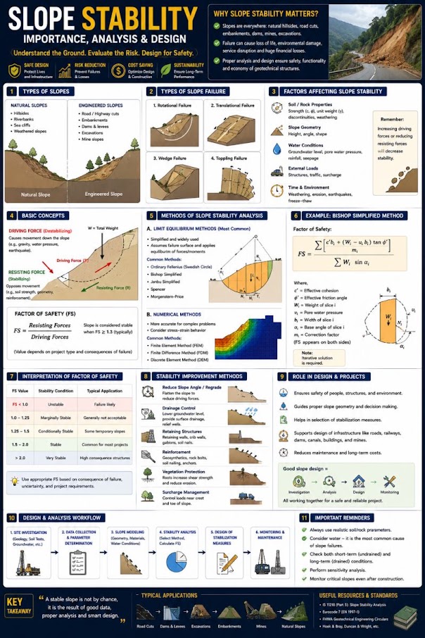
| Earthwork | Material | Slope |
|---|---|---|
| Cut | Silt | 2.5–3 : 1 |
| Cut | Muddy (silty) sand | 2–3 : 1 |
| Cut | Gravel | 1.5–2 : 1 |
| Cut | Stable clay | 1–1.5 : 1 |
| Embankment | Usual soils | 1.5–2 : 1 |
| Embankment | Gravel, sand | 2 : 1 |
| Embankment | Erosion-prone soils | 2 : 1 |
Values quoted by Profillidis from Bowles. Starting points only; the factors of safety in this chapter govern.
Profillidis emphasizes studying the geological formation along a cut, especially its joint pattern, so as to disturb the existing equilibrium as little as possible; protecting slopes with vegetation; providing slope drainage to prevent softening; and checking the foundation beneath an embankment as well as the fill. Where the ground slope exceeds 1:10, he recommends benching the embankment base (Chapter 3, §3.2).
After Profillidis (2014), §9.12; values after Bowles (2001). Full reference under Supplemental Sources.
Values from these correlations are estimates, not test results. State the equation ID and source when one is used, confirm the soil or rock is within its range, and calibrate against site testing before design.
Railroad slopes exhibit four primary failure modes that drive the selection of analytical method:
Reference graphics


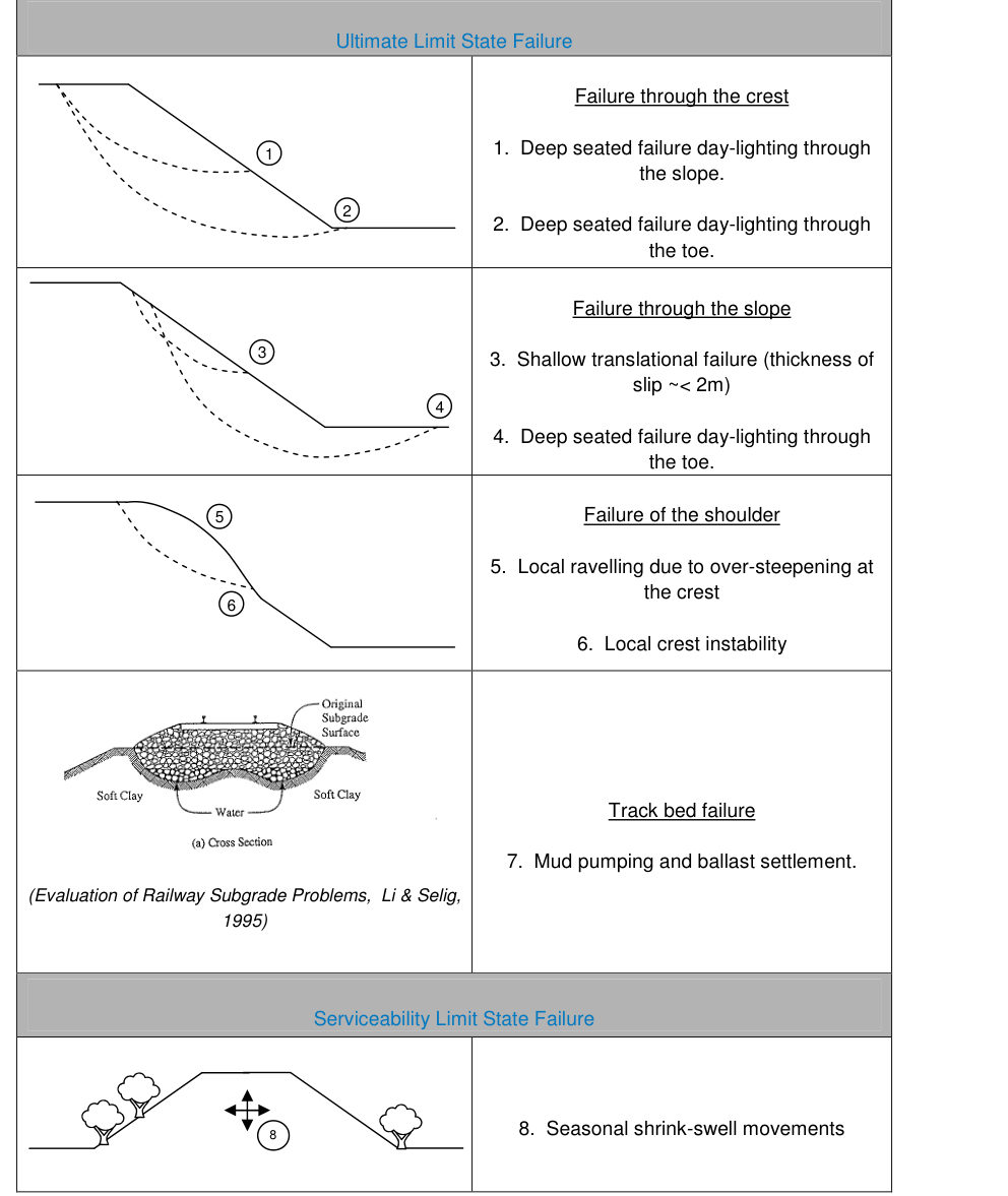
Network Rail’s review of embankment failures (August 2003 – December 2009), carried out for RSSB, separates mechanisms by how much railway traffic contributes (Figure 13-S1):
Table 13-S1. Common embankment failure mechanisms and the role of traffic (RSSB 1386, Table 2.1, condensed)
| Mechanism | Impact on track | Traffic influence | Likely triggers |
|---|---|---|---|
| Deep-seated failure through/below toe, daylighting next to track | Catastrophic | Small | Loss of shear strength, high pore pressure |
| Deep-seated failure daylighting on the slope | Small lateral/vertical deformation | Small | Loss of shear strength, high pore pressure |
| Shallow slips daylighting near the crest | Small to medium; loss of lateral support | Small to medium | Tension cracks, seasonal deformation, high pore pressure |
| Unravelling of ballast/ash shoulder | Excessive deformation | Large | Vibration, dry summer |
| Shear failure through fill below ballast | Small to catastrophic | Large | Heavy traffic, high pore pressure |
| Plastic deformation of fill; subgrade failure (e.g., ballast pumping) | Local subsidence, loss of support | Large | Heavy or more frequent traffic, high pore pressure |
| Seasonal shrink–swell (high-water-demand trees) | Small to medium | Small | Dry summer |
| Wash-out | Small to catastrophic | Small | Surface flow, erosion channels |
Key findings: ultimate-limit-state slips peaked in winter (wet ground), serviceability failures in late summer (desiccation), and failures were concentrated in medium- to high-plasticity fills. No correlation was found between large catastrophic failures and changes in traffic loading. Instead, traffic produces a fatigue-type mechanism that shows up as rising maintenance and poor trackbed performance rather than as a reported slip, so track maintenance records are the best indicator. The report also flags embankment–structure transitions and “hard spots” (culverts, walls) as stress concentrators that deserve more attention than they have received. Its preliminary models used only the static axle load, citing literature that the dynamic component is negligible at moderate speeds.
Source: Mott MacDonald (2011). The Effects of Railway Traffic on Embankment Stability. RSSB Research Project 1386 (Revised), Rail Safety and Standards Board
| Category | Field signature | Typical response |
|---|---|---|
| 1.1 Scarp far below track | Tension crack on lower slope; shallow creep shown by leaning poles, fences, trees | Walk the slope; monitor and plan mitigation |
| 1.2 Scarp at shoulder | Crack in or at the toe of ballast; surfacing and cross-level defects | Instability retrogressing toward the track; investigate and act |
| 1.3 Scarp directly below track | Main slide body at ballast level; slow or rapid | Drainage/subdrainage, geometry (flatten, berm, divert) or structure (walls, nails) |
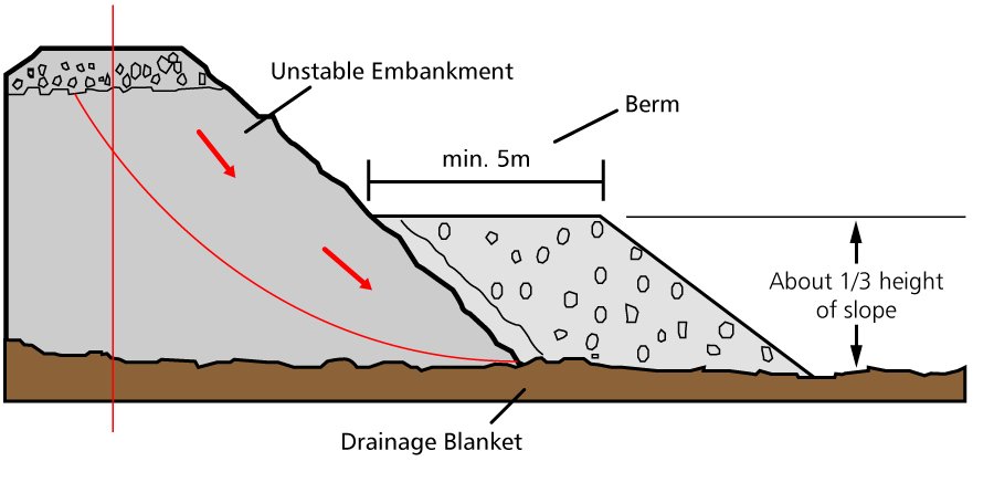
| 1.4 Scarp uphill of track (very deep) | Cross-level drops toward the high side | Large toe berm about 1/3 of slide height; walls do not work |
| 2.1 Uphill toe falling on or pushing track | Crack far above; toe bulge in ditch | Gravity or anchored wall; dewatering |
| 2.2 Uphill toe heaving track | Track lifted and shifted sideways | Gravity or anchored wall; dewatering |
| 2.4 Slide taking track down | “Whole hill moving”; up to about 60 ft deep; reactivated old slides | Very difficult; major engineering |
Figures · click to zoom
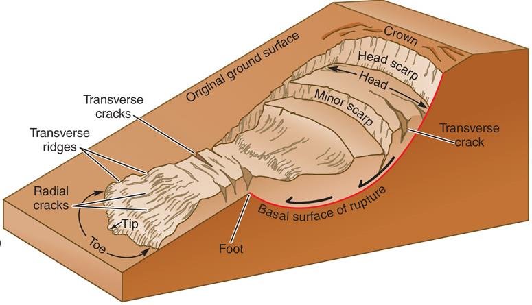
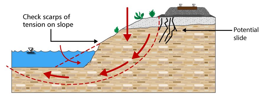
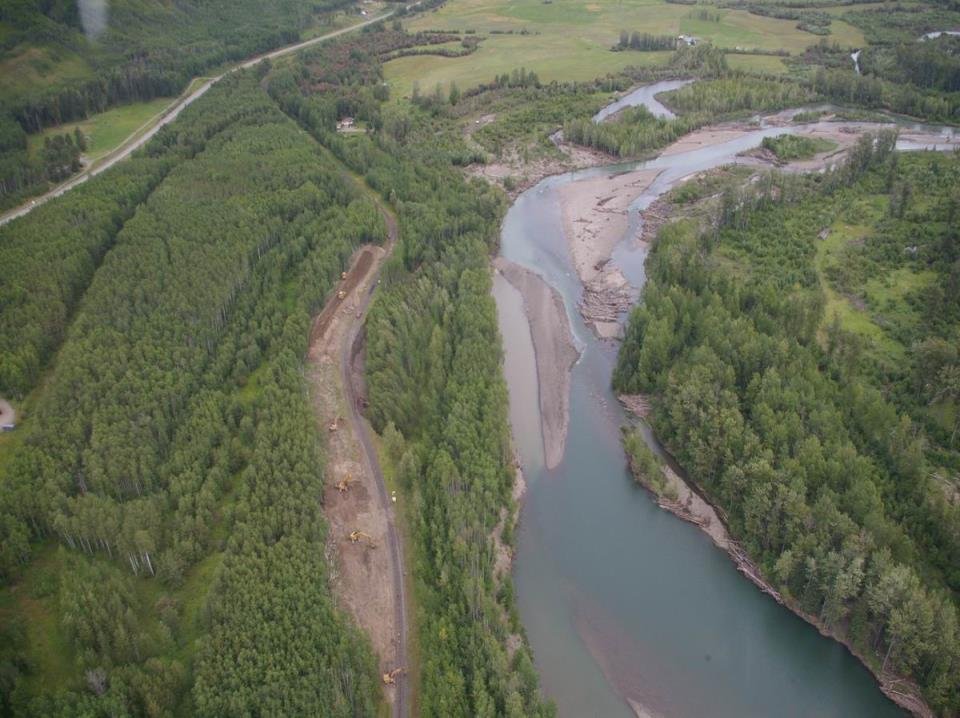
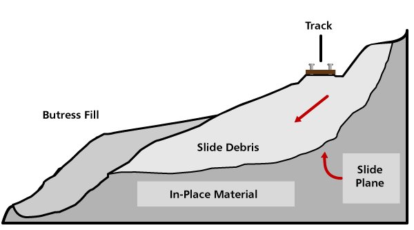
After Geotechnology for Railroaders Program, Module 5; §03–07. Full reference under Supplemental Sources.
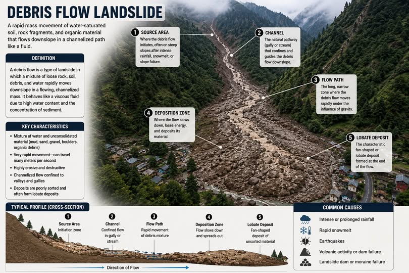
Failures on operating lines fall into four locations, each with its own usual trigger and fix:
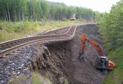
Sidehill fills are the most critical. They slide through the fill or the natural hillside soil, often long after construction, and the trigger is commonly a change in drainage. Correct the drainage before failure, not after.
Train load in stability analysis. A loaded 100-ton car is roughly 1,400 psf over the 8.5-ft tie length. Embankment geometry reduces the track’s bearing factor of safety by up to about 30% compared with flat ground (Chapter 11, Table 11-SW1).
After Selig & Waters (1994), chs. 10 and 11. Full reference under Supplemental Sources.
All limit equilibrium methods divide the failure mass into vertical slices and apply static equilibrium to the slice forces. They differ in which inter-slice forces they include and which equilibrium equations they satisfy:
| Method | Satisfies Moment Eq. | Satisfies Force Eq. | Inter-Slice Forces | Best Use |
|---|---|---|---|---|
| Ordinary (Fellenius) | Yes (moment) | No | Neglected | Quick check only; underestimates FS |
| Bishop Simplified | Yes | Vertical only | Horizontal only | Circular surfaces, most railroad practice |
| Janbu Simplified | No | Yes | Horizontal only | Non-circular; requires correction factor |
| Janbu Generalized | Yes | Yes | Full (specified) | Non-circular, compound |
| Spencer | Yes | Yes | Constant inclination | Rigorous; all surface types |
| Morgenstern-Price | Yes | Yes | Variable (f(x)) | Most rigorous; CSXT/Amtrak complex cases |
Reference graphics
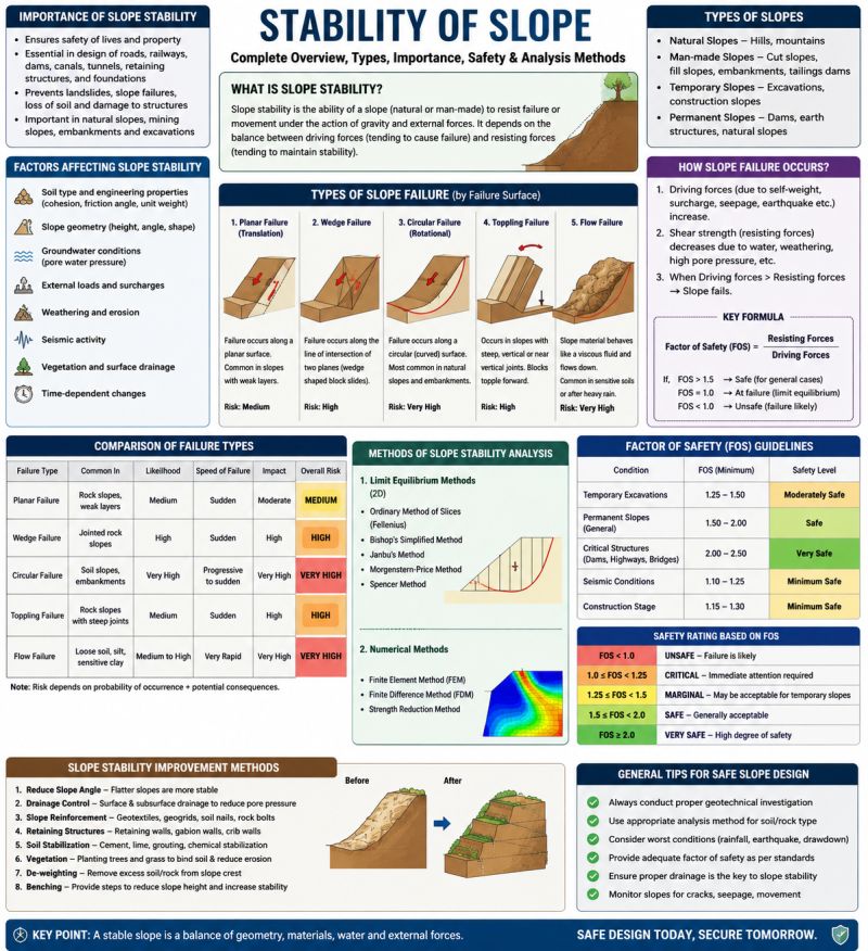

The Bishop Simplified method (1955) satisfies overall moment equilibrium and vertical force equilibrium for each slice. It is the standard method for circular failure analysis in railroad embankment design.
For a failure mass divided into n vertical slices, each of width b and height h at its center:
FS = Σ [1/mα,i · (c'i·bi + (Wi − ui·bi) tan φ'i)] / Σ Wi·sin αi
mα,i = cos αi · [1 + (tan αi · tan φ'i) / FS]
Where:
Because FS appears on both sides of Equation 13-1, the solution is iterative: assume FS, compute m_α, compute new FS, repeat until convergence (typically 3–5 iterations).
Wi = γavg,i · hi · bi · 1 ft (per unit width, kips/ft or lb/ft)
Where γ_avg,i = weighted average unit weight of materials in slice i (pcf); h_i = average slice height (ft).
For preliminary and parametric analysis, pore pressure is expressed as a fraction of total overburden:
Reference graphics
ru = u / (γ · h) = pore pressure / total vertical stress
Typical r_u values: 0 for fully drained slope; 0.25–0.35 for partially drained embankment fill; 0.50 for steady-state seepage with phreatic surface at the slope surface (worst case). USACE EM 1110-2-1902 specifies that steady-state seepage with drawdown must be analyzed separately from the static long-term case.
For a planar or compound failure surface, Janbu Simplified satisfies horizontal force equilibrium:
FS = f₀ · Σ [1/nα,i · (c'i·li + (Wi − ui·bi)·tan φ'i)] / Σ Wi·tan αi
nα,i = cos²αi · [1 + (tan αi · tan φ'i)/FS]
f₀ = 1 + b1 · [d/L − 1.4(d/L)²]
Where d = maximum depth of failure surface below a chord connecting the crest and toe (ft); L = horizontal distance of the failure surface (ft); b1 = 0.31 for φ' > 0 soils; 0.50 for φ' = 0 (undrained clay). f₀ corrects for inter-slice shear forces neglected in the simplified formulation.
In cohesive soils, a tension crack develops at the crest of the failure mass to a theoretical depth:
zc = 2c' / (γ · √Ka) = 2su / γ (for φ' = 0, undrained)
Where K_a = tan²(45 − φ'/2). For φ' = 0: z_c = 2s_u / γ. The tension crack reduces the effective length of the failure arc and, when water-filled, adds a destabilizing hydrostatic pressure. USACE EM 1110-2-1902 requires that tension crack analysis be performed for all embankments and cuts in cohesive soils with the crack assumed water-filled in the critical stability case.
Water pressure in tension crack:
Pw = 0.5 · γw · zc² (lb/ft, acts horizontally into failure mass)
EM 1110-2-1902 recommends the infinite slope method for slopes of cohesionless material, where the critical surface lies parallel to and just below the face. With c′ = 0, slope angle β and ru = u/γz:
F = (cos2β − ru) tan φ′ / (cos β sin β)
A circular search in the same material converges on a very shallow, large-radius circle with the same FS. USACE cautions that the lowest FS is often such a shallow surface, while deeper surfaces carry the real consequence. For a granular embankment over soft clay, report the deeper surfaces that could take out the track even when a skin slide has a lower FS. In the other direction, shallow fully-softened slides in clay fills (above) are exactly the ones that undercut ballast shoulders.
Source: U.S. Army Corps of Engineers (2003). Slope Stability. EM 1110-2-1902
For railroad slopes in seismically active regions (UPRR western network, BNSF Cascades/Rockies, CPKC Rockies, Amtrak NEC through New York/Connecticut), a pseudo-static horizontal force is applied to the failure mass to represent earthquake loading.
Feq = kh · W
Where:
The pseudo-static force F_eq is added to the driving moments/forces in the Bishop or Janbu equations. USACE EM 1110-2-1902 specifies minimum FS = 1.0 for pseudo-static analysis (the slope should not fail during the design earthquake, even with zero reserve). BNSF EI requires FS ≥ 1.1 pseudo-static.
FS = Σ [1/mα,i · (c'i·bi + (Wi − ui·bi)·tan φ'i)]
/ Σ (Wi·sin αi + kh·Wi·cos αi · Rm/R)
Where R = failure circle radius (ft) and R_m = moment arm for the pseudo-static force (approximately equal to the height of the centroid of the failure mass above the center of the circle).
USACE EM 1110-2-1902 (2003) provides the standard minimum FS criteria used across all nine railroad clients as a baseline:
| Loading Condition | USACE Min FS | CSXT ES | NSR ESM | BNSF EI | Amtrak ES | G&W EB | CPKC TS | CN ES |
|---|---|---|---|---|---|---|---|---|
| End-of-construction (undrained) | 1.3 | 1.3 | 1.3 | 1.4 | 1.5 | 1.3 | 1.3 | 1.3 |
| Long-term static (drained) | 1.5 | 1.5 | 1.5 | 1.5 | 1.75 | 1.3–1.5 | 1.5 | 1.4 |
| Steady-state seepage | 1.5 | 1.5 | 1.5 | 1.5 | 1.75 | 1.4 | 1.5 | 1.4 |
| Rapid drawdown | 1.3 | 1.3 | 1.3 | 1.3 | 1.5 | 1.3 | 1.3 | 1.3 |
| Pseudo-static seismic | 1.0 | 1.1 | 1.0 | 1.1 | 1.1 | 1.0 | 1.1 | 1.0 |
| Residual (progressive failure) | 1.2 | 1.3 | 1.2 | 1.3 | 1.5 | 1.2 | 1.2 | 1.2 |
| Emergency repair (temporary) | 1.1 | 1.1 | 1.1 | 1.1 | 1.3 | 1.1 | 1.1 | 1.1 |
Client-specific deviations from USACE baseline reflect the consequence of failure on high-density operations. Amtrak's FS = 1.75 for long-term static reflects the catastrophic consequence of a slope failure under a 125 mph Acela Express.
Table 13-1 lists a “USACE Min FS” column, but EM 1110-2-1902 prescribes values only for new earth and rock-fill dams (Table 3-1): 1.3 at end of construction (including staged construction), 1.5 for long-term steady seepage, 1.4 at maximum surcharge pool, and 1.1–1.3 for rapid drawdown (1.1 from maximum surcharge pool, 1.3 from maximum storage pool; 1.4–1.5 where drawdown is routine, as in pumped storage). The manual does not tabulate pseudo-static, residual or emergency-repair values; for earthquake loading it refers to ER 1110-2-1806. Cite those rows to the client standards or to project-specific judgment, not to USACE.
For “other slopes” — and EM 1110-2-1902 names railway embankments explicitly — USACE says FS should reflect both the uncertainty in strength and pore pressure and the consequence of failure. Where both are small, about 1.3 or even less can be acceptable. Where either grows, a larger FS is needed, and “large uncertainties coupled with large consequences of failure represent an unacceptable condition, no matter what the calculated value of the factor of safety.” Typical minimums are about 1.3 for end of construction and multistage loading, 1.5 for long-term loading, and 1.1–1.3 for infrequent rapid drawdown.
Cuts get weaker with time. For excavated slopes, the long-term condition is normally critical because pore pressures rise and the soil swells and weakens after excavation. A cut in low-permeability soil can stand temporarily yet be unstable in the long term; USACE calls this inherently dangerous and allows it only with detailed study and the observational method.
Source: U.S. Army Corps of Engineers (2003). Slope Stability. EM 1110-2-1902
In overconsolidated clays and clay shales, the post-failure (residual) strength is significantly lower than peak strength. The residual friction angle φ'_r is measured by ring shear test (ASTM D 6467) or repeated direct shear at large displacement.
Reference graphics

τ_r = c'_r + σ'_n · tan φ'_r
For Cretaceous clay shales (CPKC prairie territory; NSR Pocahontas district): c'_r ≈ 0 psf; φ'_r = 8°–14° (Skempton 1985; ring shear data). This is dramatically lower than peak φ' = 24°–30°, meaning a slope designed at FS = 1.5 using peak strength may fail over decades at FS < 1.0 using residual strength as progressive straining reduces the mobilized angle along the surface.
CPKC TS requires that all cut slopes in clay shale be analyzed using residual strength parameters with FS ≥ 1.2 minimum. NSR ESM requires the same in Appalachian shale territory. The consultant must confirm whether the soil has experienced previous shearing (by identifying pre-existing slickensides in core samples or split spoon) — if slickensides are present, residual strength governs.
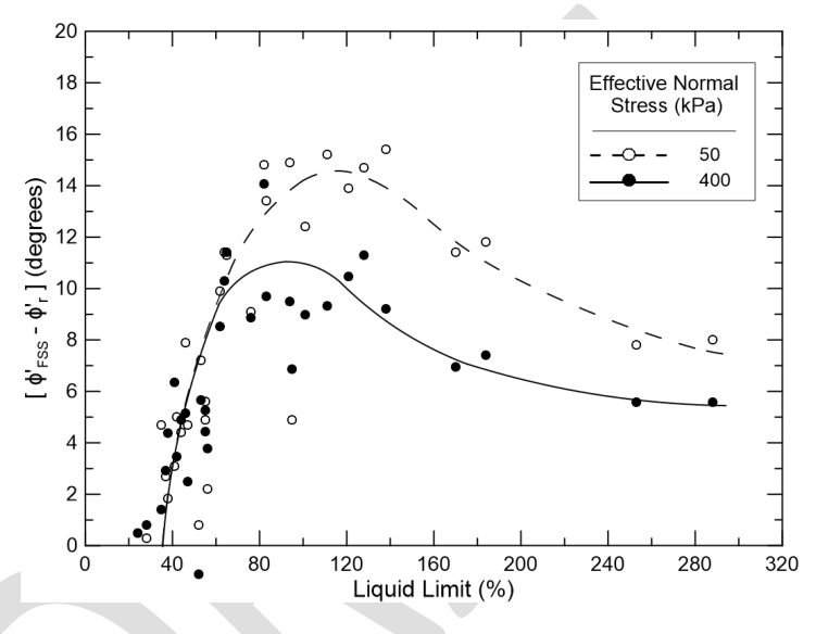
Section 13.6 moves directly from peak to residual strength. The intermediate fully softened strength (FSS) — close to the peak strength of the soil in a normally consolidated state — is the one that governs first-time slides in two situations common on railroads: (1) cuts in overconsolidated, fissured clays and clay shales, and (2) compacted clay embankments exposed to wet–dry cycles. The USACE/ASCE white paper notes that 3H:1V–4H:1V slopes 15–25 ft high routinely compute FS > 1.5 (often > 2) with peak strengths, yet many have failed, implying FS ≈ 1. One case describes a compacted fill slope that failed after about six years on a shallow surface, with back-analysis matching the FSS.
Source: Stark, T. D. et al. (2016). Development and Use of Fully Softened Shear Strength in Slope Stability Analyses, Third Draft. USACE / ASCE FSS Subcommittee
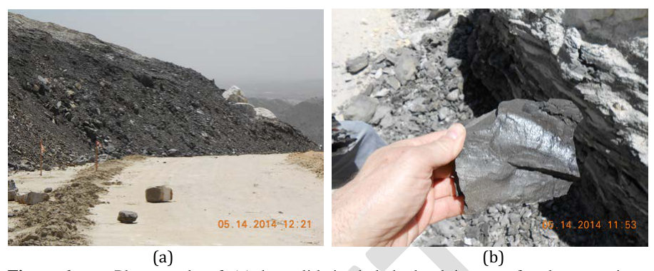
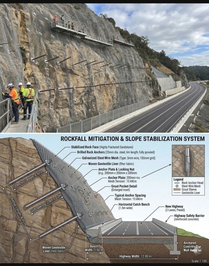
For rock cut slopes along NSR Appalachian routes, BNSF Montana/Idaho territory, and CPKC Rocky Mountain corridor, kinematic analysis of joint and bedding plane orientations governs slope geometry over soil mechanics methods.
Reference graphics

FS = (c'_j · A + (W·cos αp − U − V·sin αp) · tan φ'_j)
/ (W·sin αp + V·cos αp)
Where:
| Rock Type | c'_j (psf) | φ'_j (°) | Notes |
|---|---|---|---|
| Clean sandstone joint | 0–500 | 28–35 | NSR WV, BNSF MT |
| Clay-filled shale parting | 0–200 | 8–16 | NSR/CPKC clay shale; use residual |
| Limestone bedding plane | 0–1,000 | 32–40 | G&W Gulf Coast carbonate |
| Granite exfoliation joint | 0 | 35–42 | UPRR Sierra Nevada |
| Weathered basalt | 0–500 | 25–32 | BNSF Pacific Northwest |
Kinematic feasibility of planar, wedge, and toppling failure must be evaluated by stereographic projection (stereonet analysis) using joint orientation data collected during field mapping. This analysis is beyond scope here but must be performed for every rock cut slope on NSR, BNSF, and CPKC projects per their respective standards.
Section 13.7 leaves stereonet analysis out of scope. The screening rules are short enough to apply to every railroad rock cut. Following Wyllie and Mah (2004), with face dip ψf and dip direction αf:
Wyllie and Mah note it is rarely possible to change an alignment enough to avoid an adverse structure; the choice is usually to flatten that face or reinforce it.
A California study of 308 highway rock falls (McCauley et al., 1985, reported by Wyllie and Mah) found that water-related causes account for 68% (rain 30%, freeze–thaw 21%, snowmelt 8%, channeled runoff 7%, plus differential erosion, springs and tree roots), and 85% when adverse geology is added. On a major western Canadian railroad, about 70% of 25 years of recorded falls occurred in winter, and falls smaller than about 1.3 yd³ occurred up to 50 times a year, while 13,100 yd³ slides recurred every 10–50 years. Many railroad cuts were blasted more than a century ago with techniques that damaged the rock, and have since weathered. Schedule scaling and inspection for late fall and early spring, and treat drainage as a primary rock-fall control.
Source: Wyllie, D. C. and Mah, C. W. (2004). Rock Slope Engineering: Civil and Mining, 4th ed. Spon Press
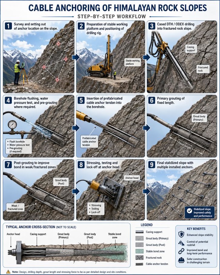
Active high-tensile mesh. Draped mesh only guides falling rock to the ditch; a pretensioned mesh pinned with a grid of soil or rock nails actively holds the surface layer. The Geobrugg TECCO system (presented at the Appalachian geohazards conference) uses wire of more than 256 ksi, giving mesh tensile strength of about 10.2 kips/ft, compared with about 3 kips/ft for common steel wire mesh and 2.75 kips/ft for a PET geogrid. The design (RUVOLUM concept) checks (1) sliding of the surface layer parallel to the slope and (2) local failure between nails, and sets the maximum nail spacing. It does not replace a global stability analysis (e.g., Bishop) of deeper surfaces. The presentation cites failed alternatives — shotcrete facing replaced after about 10 years and soft geogrid facing that failed by creep, cutting at sharp edges and overload.
Load transfer in grouted bolts and cables. Wang, Hagan and Cao (2016) summarize laboratory work on fully grouted reinforcement:
Source: Amend, F. Slope Stabilization with High Tensile Wire Mesh. Geohazards in Transportation in the Appalachian Region Conference, Geobrugg North America · Wang, S., Hagan, P. C. and Cao, C. (2016). Advances in Rock-Support and Geotechnical Engineering. Butterworth-Heinemann
| Strategy | Methods | Notes |
|---|---|---|
| Stabilizing | Drainage, trimming, scaling, shotcrete, bolting; retaining walls; stabilizing berms; horizontal drains | Highest safety and reliability impact; cost varies; scaled-rock disposal can be a problem |
| Protecting | Catchment nets; barrier walls; lock blocks; rock sheds (~$1–10M); tunnels (~$3–50M); flumes (~$600K); rock mesh (~$100–250K) | Nets for confined chutes and unscalable sources; keep catch ditches and wall accumulation zones clean |
| Warning | Slide-detector fences; mercury and tip-over switches; temporary radio units | A warning layer, not a fix: about 90% of trips prove passable; maintenance burden and false positives |
A Jasper near-miss shows the limit of warning devices: the fence tripped as designed, but the train could not stop on the grade. Use engineering-grade concrete for lock blocks and source matching keys. Mark already-documented fallen rocks with an X.
Figures · click to zoom
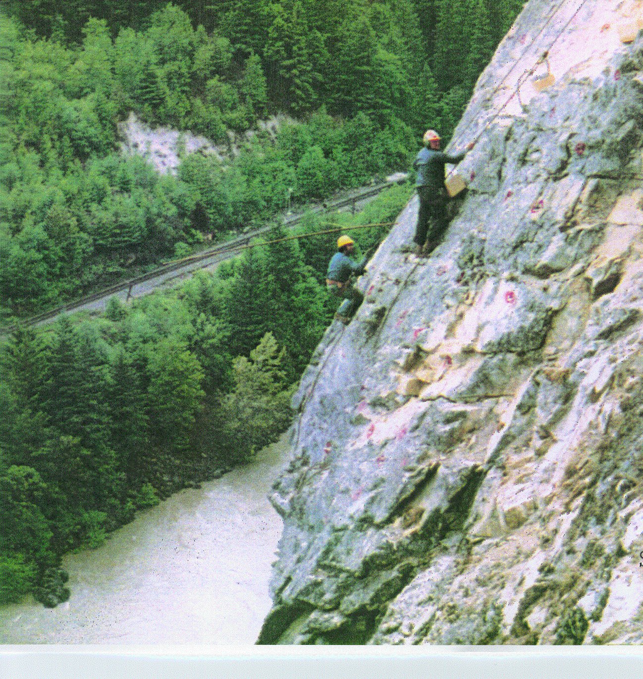
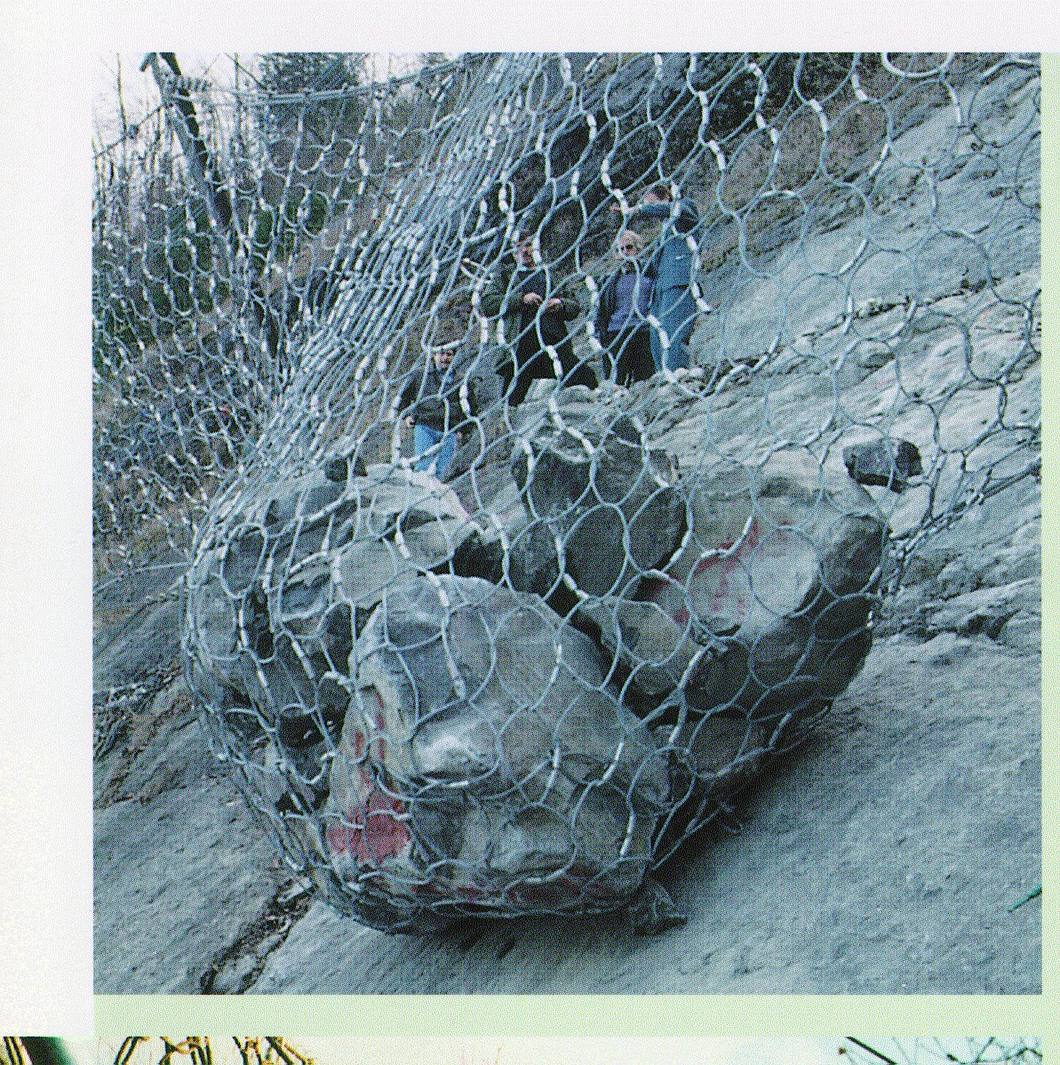
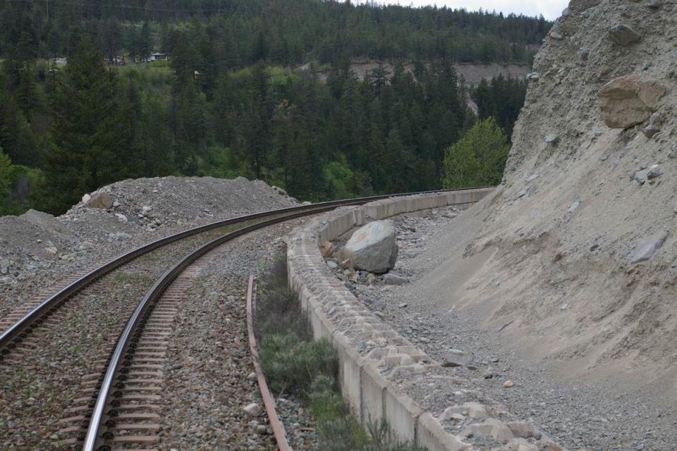
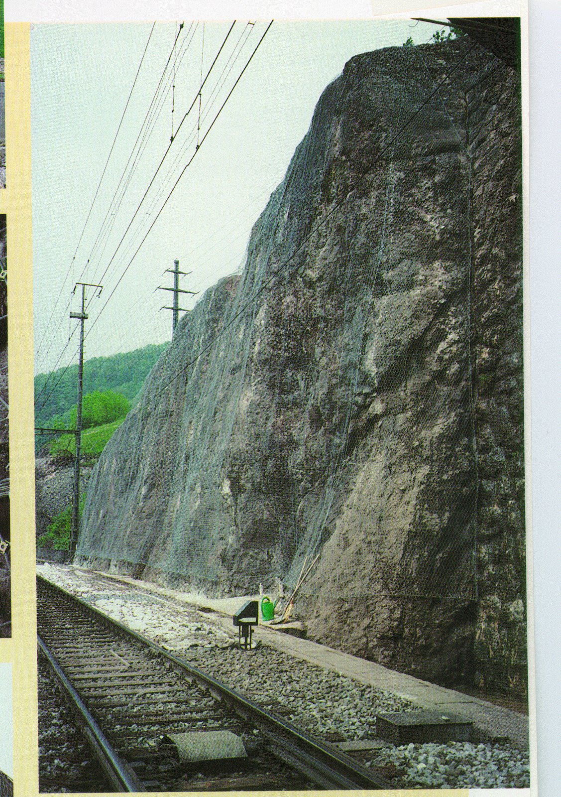
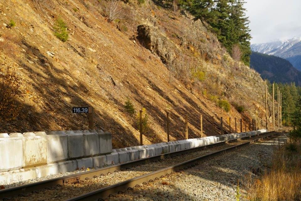
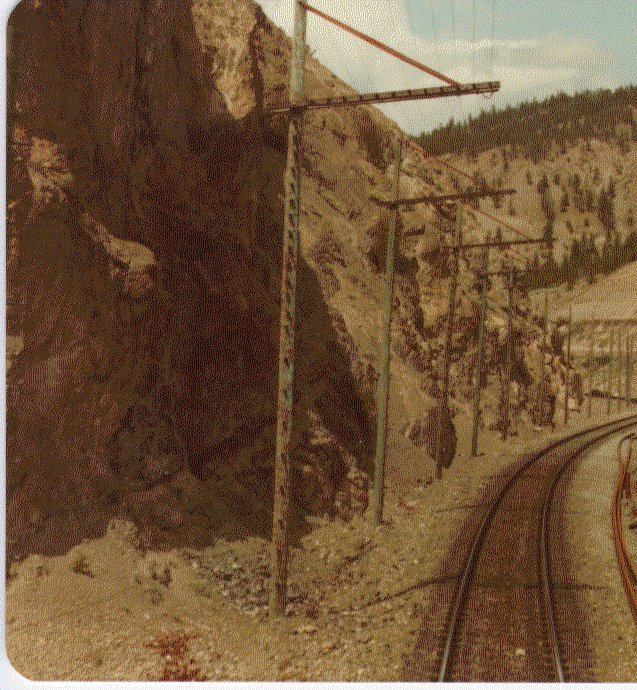
After Geotechnology for Railroaders Program, Module 6.4; §02–04. Full reference under Supplemental Sources.
UPRR Missouri River territory and BNSF river crossing embankments are subject to rapid drawdown — when a river in flood recedes quickly, the phreatic surface within the embankment lags behind the external water level, creating a destabilizing outward seepage gradient.
The three-stage approach per USACE EM 1110-2-1902 Appendix F:
For materials with k > 10⁻³ ft/day (sands and gravels), drained strengths can be used at the lowered pool because drainage occurs faster than drawdown. For clays with k < 10⁻⁵ ft/day, CU strengths apply throughout.
While a pond is high, its weight helps hold the slope despite saturation. When it drops quickly, that support disappears while the fill is still saturated, and seepage reverses outward. Field guidance is that the slope stays at its least stable for about 12 hours after drawdown, recovering over 12–24 hours as the bank drains. Monitor for at least that long, and for at least three days where the drop is 2 ft or more. Beaver-dam or culvert releases create the same condition. The Nakina derailment of 1992, in which two employees were killed, was a rapid-drawdown failure beneath a moving train.
Figures · click to zoom
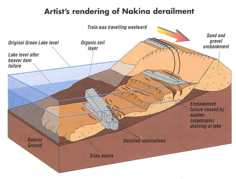
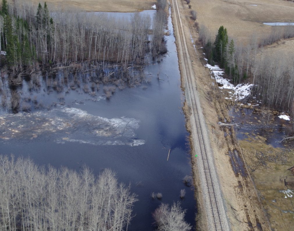
After Geotechnology for Railroaders Program, Module 7.1, Module 4, Module 6.5; Module 7.1 §06; Module 4 §10. Full reference under Supplemental Sources.
Case study: 13.16.1 Flood drawdown failures along the Brisbane River (Look 2023), in §13.16 Case Studies.
| Client | Territory | Soil/Rock | c' (psf) | φ' (°) | φ'_r (°) | γ (pcf) | s_u (psf) | Design FS |
|---|---|---|---|---|---|---|---|---|
| CSXT | Coastal GA/SC | Soft CH clay foundation | 0 | — | — | 100–105 | 400–800 | ≥1.3 (EOC) |
| NSR | WV Pocahontas | Residual silty clay | 200 | 22 | 12 | 115 | — | ≥1.5 (LT) |
| NSR | VA Appalachian | Weathered shale | 0 | 14 | 9 | 130 | — | ≥1.2 (res.) |
| G&W | Gulf Coast LA | Soft CL/CH | 0 | — | — | 105 | 600–1,200 | ≥1.3 |
| UPRR | NE Loess | Loess (ML) | 300 | 28 | — | 110 | — | ≥1.5 |
| BNSF | MT Mountain | Dense glacial till | 500 | 32 | — | 135 | — | ≥1.5 |
| CPKC | SK Prairie | Cretaceous clay shale | 0 | 10 | 6 | 125 | — | ≥1.2 (res.) |
| Amtrak | NEC CT/NY | Stiff marine clay | 100 | 26 | — | 120 | 1,500–2,500 | ≥1.75 |
| CN | ON/QC | Leda quick clay | 0 | — | — | 115 | 200–600 | ≥1.4 (staged) |
Reference graphics
Project context: Norfolk Southern Pocahontas District, WV. Proposed 20-ft high railroad fill over residual CL soil derived from shale. Soil profile: embankment fill (c' = 100 psf, φ' = 30°, γ = 120 pcf); foundation CL residual clay (c' = 200 psf, φ' = 22°, γ = 115 pcf). Phreatic surface at 1/3 height of embankment from base. Trial circular failure surface: radius R = 38 ft; circle center 15 ft above embankment crest. NSR ESM requires FS ≥ 1.5. Divide failure mass into 5 slices.
Step 1 — Slice geometry and weights (per unit width)
| Slice | b (ft) | h_avg (ft) | Material | γ (pcf) | W = γ·h·b (lb/ft) | α (°) | u (psf) |
|---|---|---|---|---|---|---|---|
| 1 | 6 | 4.0 | Fill | 120 | 2,880 | −15 | 0 |
| 2 | 8 | 12.0 | Fill | 120 | 11,520 | 0 | 0 |
| 3 | 8 | 18.5 | Fill+Fdn | 118 | 17,464 | +12 | 375 |
| 4 | 8 | 14.0 | Fdn Clay | 115 | 12,880 | +28 | 624 |
| 5 | 6 | 6.0 | Fdn Clay | 115 | 4,140 | +42 | 0 |
Pore pressure u = γ_w × h_w: at Slices 3 and 4, h_w ≈ 6 ft and 10 ft respectively; u = 62.4 × 6 = 374 ≈ 375 psf; 62.4 × 10 = 624 psf.
Step 2 — Driving moment (Σ W_i sin α_i)
Slice 1: 2,880 × sin(−15°) = 2,880 × (−0.259) = −746 lb/ft
Slice 2: 11,520 × sin(0°) = 0
Slice 3: 17,464 × sin(12°) = 17,464 × 0.208 = 3,633 lb/ft
Slice 4: 12,880 × sin(28°) = 12,880 × 0.469 = 6,041 lb/ft
Slice 5: 4,140 × sin(42°) = 4,140 × 0.669 = 2,770 lb/ft
Σ Wi·sin αi = −746 + 0 + 3,633 + 6,041 + 2,770 = 11,698 lb/ft
Step 3 — Resisting forces — iterate to FS = 1.52 (trial)
For each slice compute m_α = cos α [1 + (tan α · tan φ') / FS]:
Using φ' = 22° (foundation) for Slices 3–5; φ' = 30° (fill) for Slices 1–2; c' = 200 psf (fdn), 100 psf (fill); assume FS = 1.52.
| Slice | c'b (lb/ft) | (W−ub) tan φ' (lb/ft) | Numerator (lb/ft) | cos α | tan α · tan φ' / FS | m_α | Num/m_α |
|---|---|---|---|---|---|---|---|
| 1 | 100×6=600 | (2,880−0)×0.577=1,662 | 2,262 | 0.966 | (−0.268×0.577)/1.52=−0.102 | 0.966×0.898=0.867 | 2,609 |
| 2 | 100×8=800 | (11,520−0)×0.577=6,647 | 7,447 | 1.000 | 0 | 1.000 | 7,447 |
| 3 | 200×8=1,600 | (17,464−375×8)×0.404=(17,464−3,000)×0.404=5,835 | 7,435 | 0.978 | (0.213×0.404)/1.52=0.057 | 0.978×1.057=1.034 | 7,190 |
| 4 | 200×8=1,600 | (12,880−624×8)×0.404=(12,880−4,992)×0.404=3,191 | 4,791 | 0.883 | (0.532×0.404)/1.52=0.141 | 0.883×1.141=1.008 | 4,754 |
| 5 | 200×6=1,200 | (4,140−0)×0.404=1,673 | 2,873 | 0.743 | (0.900×0.404)/1.52=0.239 | 0.743×1.239=0.921 | 3,120 |
Σ (Num/m_α) = 2,609 + 7,447 + 7,190 + 4,754 + 3,120 = 25,120 lb/ft
Step 4 — Computed FS
FS = 25,120 / 11,698 = 2.15
The trial FS (1.52) does not match the computed FS (2.15). This is a single-trial demonstration; in practice, the critical circle is found by systematically moving the circle center and radius to minimize FS. The minimum FS for the critical circle at this site would be reported after searching over hundreds of trial circles in SLOPE/W or SLIDE. The computed FS of 2.15 for this trial surface indicates adequate stability; the critical surface will produce a lower value. For this example, assume the critical circle yields FS = 1.72, which meets NSR ESM's FS ≥ 1.5 requirement.
Conclusion: The 20-ft embankment design with 2H:1V side slopes over the residual CL clay provides adequate long-term stability per NSR ESM. NSR requires submission of SLOPE/W output (minimum 50 trial circles) to the NSR Geotechnical Engineering group for independent review before construction authorization.
Project context: BNSF siding extension, Crescent, WA. Proposed 12-ft embankment over soft saturated CH (s_u = 700 psf undrained, γ = 103 pcf). End-of-construction (undrained) analysis required; BNSF EI requires FS ≥ 1.4 at EOC. Check 1.5H:1V embankment slopes.
Simplified φ = 0 analysis (Taylor's stability chart):
For φ' = 0 soils, the critical circular failure surface passes through the toe for D_f/H ≤ 1 (where D_f = depth of firm layer) and is characterized by the stability number N_s:
FS = Ns · su / (γ · H)
N_s is a function of slope angle β and depth factor D = D_f/H. For 1.5H:1V slope (β ≈ 34°) and no firm layer immediately below (deep failure), N_s ≈ 5.52 (from Taylor's chart, Coduto 2001).
FS = 5.52 × 700 / (103 × 12)
= 3,864 / 1,236
= 3.13 ≥ 1.4 ✓
However, the soft CH must be checked for base failure (Prandtl/Terzaghi bearing capacity of the foundation clay):
q_ult = Nc · su = 5.14 × 700 = 3,598 psf
q_applied = γ_fill × H = 120 × 12 = 1,440 psf
FS_base = 3,598 / 1,440 = 2.50 ≥ 1.4 ✓
Staged construction: If s_u were 300 psf (very soft), FS = 5.52 × 300 / 1,236 = 1.34 < 1.4. BNSF EI would require staged construction — place first 6-ft lift, wait for consolidation-induced strength gain before placing the second lift. Settlement plates and piezometers (Chapter 15) monitor the consolidation progress; the fill rate is restricted until FS ≥ 1.4 is reestablished after each stage.
Conclusion: For s_u = 700 psf, the 1.5H:1V embankment at 12 ft height provides FS = 3.13 at EOC, well above BNSF EI's 1.4 minimum. BNSF EI requires that the foundation strength be confirmed by at least two CPTu soundings at every embankment location greater than 8 ft over soft ground (Chapter 7 correlation used for s_u). If CPTu reveals zones of s_u < 500 psf, staged construction with instrumentation must be implemented.
Project context: Canadian Pacific Kansas City (CPKC) Mainline, Saskatchewan. New 25-ft railway cut in Cretaceous clay shale. Residual ring shear data: c'_r = 0 psf, φ'_r = 9°. Peak parameters: c' = 300 psf, φ' = 22°. Unit weight = 130 pcf. Water table at cut bench level (worst case). Check proposed 2H:1V cut slope (β = 26.6°) using both peak and residual strengths.
Step 1 — Infinite slope analysis for shallow translational slide (0–5 ft depth)
For a shallow translational failure along a plane parallel to the slope at depth z = 4 ft:
FS = (c' + γ'·z·cos²β·tan φ') / (γ_sat·z·sin β·cos β)
With WT at surface: γ' = γ_sat − γ_w = 130 − 62.4 = 67.6 pcf; γ_sat = 130 pcf; β = 26.6°; z = 4 ft.
Peak strength:
FS_peak = (300 + 67.6×4×cos²26.6°×tan22°) / (130×4×sin26.6°×cos26.6°)
= (300 + 67.6×4×0.797×0.404) / (130×4×0.447×0.894)
= (300 + 87.1) / (207.8)
= 387.1 / 207.8 = 1.86 ≥ 1.5 ✓ (peak)
Residual strength (c'_r = 0, φ'_r = 9°):
= (67.6×4×0.797×0.1584) / 207.8
= 34.2 / 207.8 = 0.165 << 1.0 ✗
Step 2 — Interpretation
The residual strength analysis yields FS = 0.165 — the slope is in a state of impending failure at residual. This is the well-known behavior of clay shale slopes: they appear stable at first cut but fail progressively over months to years as weathering and swelling reduce the mobilized strength toward residual. CPKC TS requires that cut slopes in clay shale be designed with either: (a) gentle slopes (4H:1V to 5H:1V) that achieve FS ≥ 1.2 at residual, or (b) engineered drainage (horizontal drains) to reduce pore pressures to near-zero, or (c) slope reinforcement (soil nails, piles) to maintain stability.
Step 3 — Required slope angle for FS = 1.2 at residual (c'_r = 0)
For infinite slope with c' = 0:
This is impractically flat for a 25-ft deep railway cut.
Conclusion: Drainage is the most economical solution — reduce pore pressures by installing horizontal drains at the slope face. With u = 0 (fully drained): γ = 130 pcf (no buoyancy reduction), γ_sat replaced by γ in both numerator and denominator:
Even fully drained, FS < 1.0 at residual for a 2H:1V cut in this clay shale. A 3.5H:1V slope is the practical minimum for FS = 1.2 at residual with full drainage:
tan β = tan(9°)/1.2 = 0.132
β = 7.5° → 3H:1V + berms at 15-ft height intervals
CPKC TS requires geotechnical instrumentation (surface monuments, inclinometers) for all clay shale cuts exceeding 15 ft depth, with annual monitoring and reporting to CPKC Track Geometry Engineering.
Reference graphics

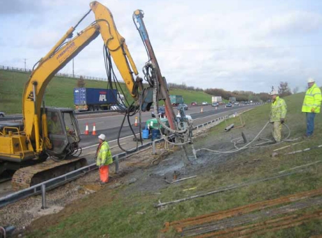
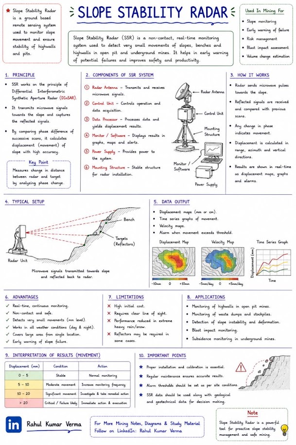
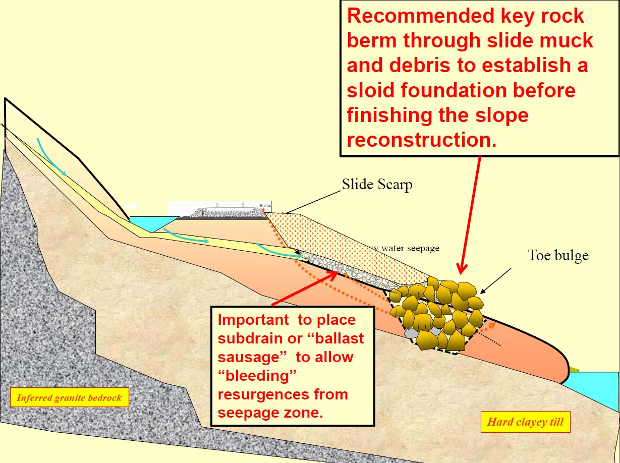
Consider remedial measures in this order: (1) drainage and subdrainage; (2) geometry, meaning a toe berm, flattening or moving the track; (3) structural support; (4) improving soil properties. Warning devices supplement these.
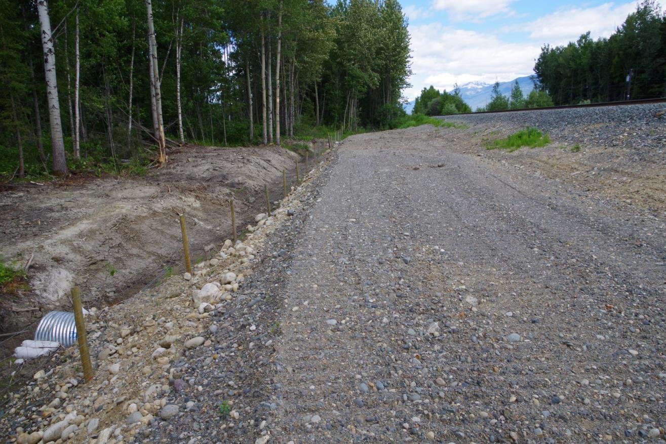
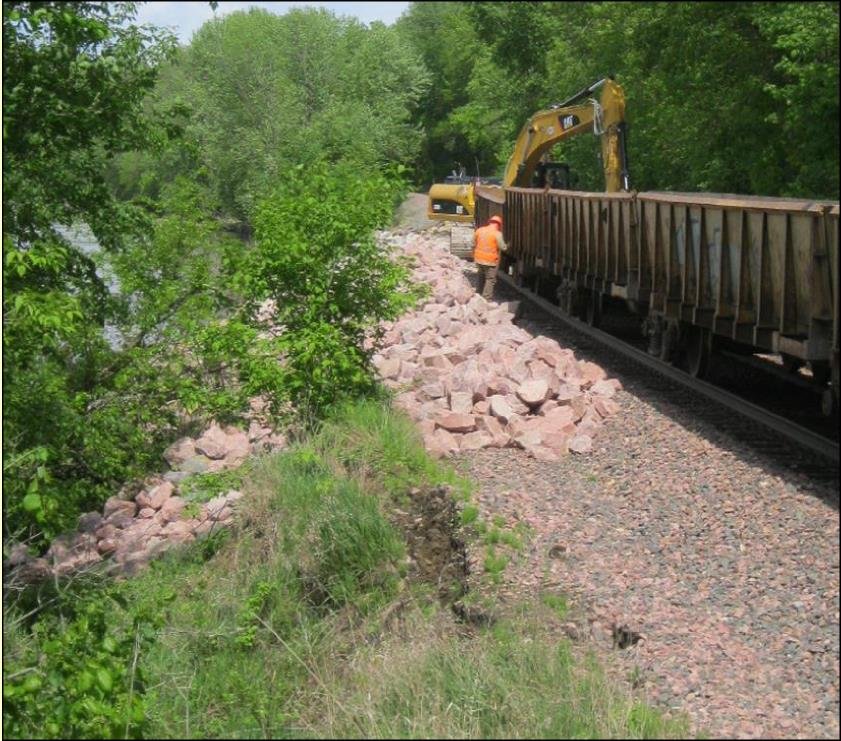
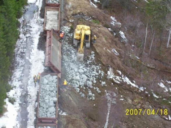
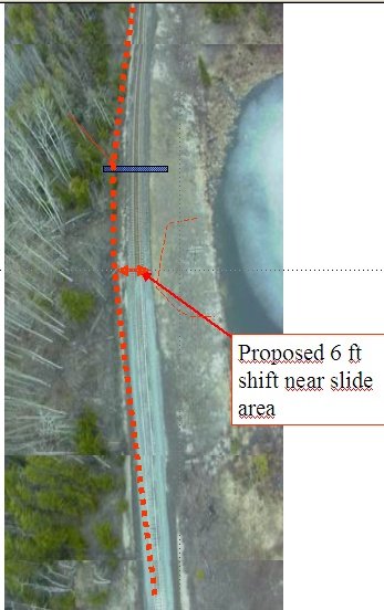
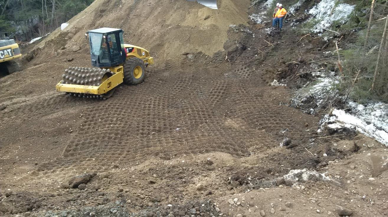
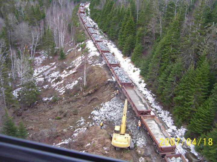
PG Sub Mile 445.7 (April 2013) is typical of most slides seen along the track. Snowmelt ran down small gullies, disappeared into the fill, raised pore pressure and took out the embankment. The repair keyed in a toe, rebuilt a 2:1 slope about 50 ft high from air-dumped fill, and added culverts.
Figures · click to zoom
After Geotechnology for Railroaders Program, Module 6.1, Module 7.1; Module 6.1 §02–04; Module 7.1 §05. Full reference under Supplemental Sources.
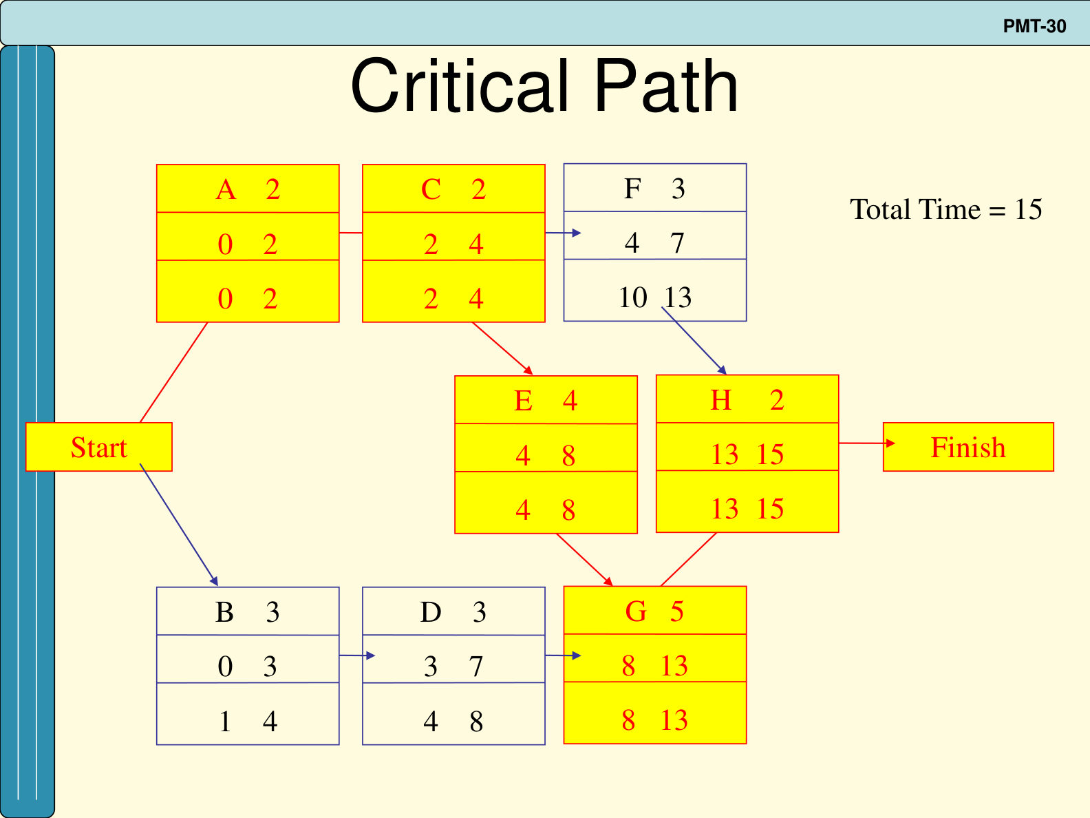
PERT handles uncertain durations by asking for three estimates per activity: optimistic a, most likely m and pessimistic b. A beta distribution gives the expected time t = (a + 4m + b) ÷ 6 and variance σ² = [(b − a) ÷ 6]². A forward pass gives the early start and finish (ES = largest EF of the predecessors; EF = ES + t), and a backward pass gives the late times (LF = smallest LS of the successors; LS = LF − t). Slack is LS − ES; activities with zero slack form the critical path. Project variance is the sum of the variances of the critical activities. Treating completion time as normally distributed, the probability of finishing by deadline D follows from Z = (D − T) ÷ σ.
Table 13-PM1. Worked example time estimates, weeks (after Swearingen n.d., slide PMT-17)
| Activity | a | m | b | t | σ² | Slack |
|---|---|---|---|---|---|---|
| A | 1 | 2 | 3 | 2 | 0.11 | 0 |
| B | 2 | 3 | 4 | 3 | 0.11 | 1 |
| C | 1 | 2 | 3 | 2 | 0.11 | 0 |
| D | 2 | 4 | 6 | 4 | 0.44 | 1 |
| E | 1 | 4 | 7 | 4 | 1.00 | 0 |
| F | 1 | 2 | 9 | 3 | 1.78 | 6 |
| G | 3 | 4 | 11 | 5 | 1.78 | 0 |
| H | 1 | 2 | 3 | 2 | 0.11 | 0 |
In the slides’ example, a foundry has 16 weeks to install a pollution-control system. The critical path A–C–E–G–H gives T = 15 weeks with variance 3.11, so σ = 1.76 weeks. Then Z = (16 − 15) ÷ 1.76 = 0.57, which corresponds to about a 71.6% chance of meeting the deadline.
For railroad work: slope repairs often have to be finished before a wet season, a freeze-up or a planned outage. Use wide pessimistic estimates for activities controlled by subsurface conditions, such as soldier pile or anchor drilling in uncertain rock, dewatering, or excavation below the slide plane. Use narrow ranges for routine tasks. If the computed probability is low, change the plan (more rigs, a second shift, a staged repair that restores track first) instead of only reporting the risk. The method assumes a single critical path. Where a near-critical path also carries large variance, the true chance of finishing on time is lower than the calculation shows, so check those paths as well.
Source: Swearingen, J. (n.d.). The Basics of Project Management Techniques [lecture slides PMT-1 to PMT-40; author from document properties], slides PMT-13 to PMT-34. Summarized and paraphrased; figures reproduced for internal reference. Full reference under Supplemental Sources.
Slope design relies on expert judgment wherever data are thin, for example in the location of the failure surface, residual strength, piezometric level or the effect of a drainage fix. Cretu et al. summarize the cognitive biases that distort such judgments and how a facilitator can counter them. The overconfidence effect is the tendency to give ranges that are too narrow. One study they cite asked seven very experienced geotechnical engineers to bracket the embankment height that would fail a clay foundation, using bounds intended to have a 50 percent chance of containing the true value. None of the seven ranges captured the actual failure height. Anchoring means that the first number spoken pulls later estimates toward it. Availability means that vivid recent events seem more probable than they are. Motivational bias covers people shading estimates to protect a past position, a budget or a client relationship, and subordinates deferring to superiors in the room. Optimism bias covers people underrating threats on projects they control.
The authors give these countermeasures. Explain the biases to the group before eliciting values. Ask for the worst credible outcome first, then the best case (which may not be “nothing”), then the most likely. Push explicitly for wider bounds. Collect estimates from junior staff or consultants separately and present them to management anonymously. Show the resulting distribution on screen so the experts can confirm that it says what they meant. Base estimates on personal experience, lessons learned, outside expert opinion and empirical records, and use the empirical records first when they exist.
For railroad work: When back-analysis or design inputs rest on judgment, run a short structured elicitation and document it. This applies to the depth of a slip surface between inclinometer readings, the residual friction angle of a slickensided clay, or the water level to assume for a ditch-line slide. Ask for the worst credible case first, record low/most-likely/high values with their reasons, and carry the full range into sensitivity or probabilistic stability runs. A single “engineering judgment” value tends to understate the uncertainty in the factor of safety. Railroad staff who have watched a site for years are valuable sources. Interview them separately from their managers, and treat their recollection of the last movement as an anchor to test, not a bound.
Source: Cretu, O., Stewart, R. and Berends, T. (2011). Risk Management for Design and Construction. Hoboken, NJ: John Wiley & Sons, pp. 111–121. Summarized and paraphrased. Full reference under Supplemental Sources.
Jacob and Müller show how a change is priced when the work as bid cannot be performed as described. The approach is not to negotiate a new lump sum. Instead, the original bid calculation is reopened, and only the parts of the item that changed are replaced. The original surcharge rates are kept.
In their example, half of a 131,000 CY excavate-haul-place item (65,400 CY) turns out to be contaminated. That portion must go to an owner-designated disposal site instead of into the on-site fill. The changed item is rebuilt as follows:
The new unit price came out about 3% above the original. The change can be paid either as a new item or as a price difference applied to the affected quantity. The authors prefer the difference method, because it shows exactly which costs were added and which were dropped.
They also list follow-on effects that may need their own pricing:
Underlying this is their split between time-variable and time-fixed site costs.
Keeping the two separate in the estimate is what makes delay and disruption costs calculable later.
For railroad work: Embankment and slide repairs regularly reveal conditions that change the work after award. Examples are contaminated or fouled-ballast spoil that cannot be reused, deeper failure surfaces, and wet borrow. Repricing from the contractor’s bid build-up only works if the contract requires that build-up to be submitted or escrowed. It also needs bid items split finely enough (excavation, haul, placement, disposal) to be reopened. For delay caused by lost track windows or a slower restoration of track speed, price the time-variable site costs per day in advance. That gives the railroad and contractor an agreed basis for standby and extension costs.
Source: Jacob, D. and Müller, C. (Eds.) (2017). Estimating in Heavy Construction: Roads, Bridges, Tunnels, Foundations. Berlin: Ernst & Sohn, pp. 12–14, 205–208. Summarized and paraphrased. Full reference under Supplemental Sources.
Pratt sets two rules for measuring earthwork. First, measure in bank measure: the actual in-place dimensions, with no allowance for swell or compaction. Those factors are applied later, when the work is priced. Second, keep each excavation category and each material separate, and measure disposal of surplus as total excavation minus common backfill.
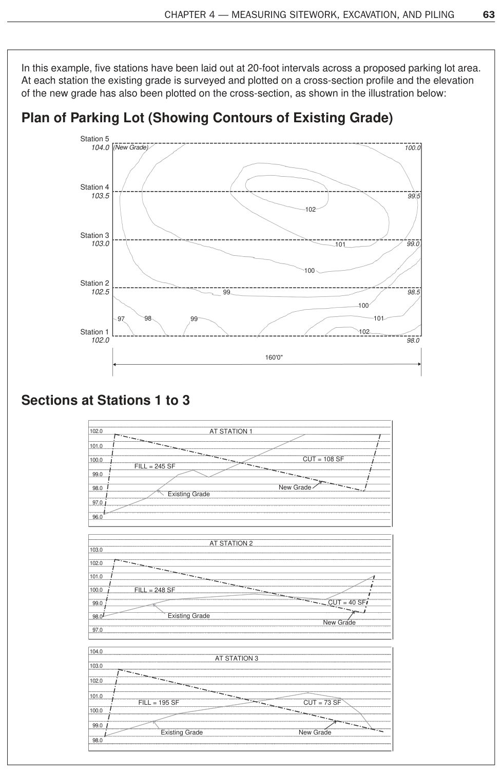
He gives two manual methods for volumes. The grid method takes the cut or fill depth at each grid node and weights it by the area that node represents: one quarter-cell at a corner, two on an edge, and four in the interior. The section method suits long, narrow work such as road and railroad construction. Cross sections are plotted at regular stations, the cut and fill areas are measured at each section, and the volumes come from the average-end-area relation:
V = station spacing × (A1/2 + AN/2 + sum of the intermediate areas)
His example uses five stations 20 ft apart. The cut areas are 108, 40, 73, 91 and 0 ft², and the fill areas are 245, 248, 195, 195 and 328 ft². That gives 5,160 ft³ (191 CY) of cut and 18,490 ft³ (685 CY) of fill. All the cut is reused, so about 494 CY of fill must be imported. Accuracy depends mainly on how faithfully the section profiles are plotted, and closer station spacing improves it.
For railroad work: a slide or washout repair is a short, long-and-narrow job of exactly this kind. A reasonable procedure is:
Each material has its own swell and compaction behavior and its own haul. Report the volumes in bank measure, state the section spacing and the survey date, and keep the section sheets in the calculation appendix. A slide that is still moving changes the existing-ground line, so the quantities will need updating before the bid.
Source: Pratt, D. J. (2011). Fundamentals of Construction Estimating, 3rd ed. Clifton Park, NY: Delmar Cengage Learning, pp. 57, 59–64. Summarized and paraphrased; figures reproduced for internal reference. Full reference under Supplemental Sources.
Checklist · Part VI · Geotechnical Analysis
Pre-Analysis
Analysis Execution
Deliverables
Question 8.1 Define the four primary failure modes for railroad slopes and describe which analysis method is most appropriate for each.
Answer: (1) Rotational circular slide — homogeneous or layered cohesive soil; Bishop Simplified or Spencer method for circular surface search. (2) Translational planar slide — failure along a discrete weak plane (bedding, shale parting, geosynthetic); infinite slope method (shallow, parallel to slope) or Janbu with a specified planar surface. (3) Compound/non-circular slide — failure surface transitions through weak layer; Janbu Generalized or Morgenstern-Price for full rigor. (4) Progressive failure — strain-softening clay or clay shale reduces mobilized strength from peak to residual over time; use Bishop or Janbu with residual strength parameters (c'_r, φ'_r from ring shear test). USACE EM 1110-2-1902 requires that the analysis method be justified in the geotechnical report based on the failure surface geometry expected for the site conditions.
Question 8.2 A railroad embankment has s_u = 500 psf in the soft foundation clay, γ_fill = 118 pcf, and a proposed fill height of 10 ft with 2H:1V slopes (β = 26.6°). Using Taylor's stability number N_s = 5.52, compute the undrained FS at end of construction. Does this meet BNSF EI's EOC minimum of FS ≥ 1.4?
Answer:
FS = Ns · su / (γfill · H)
= 5.52 × 500 / (118 × 10)
= 2,760 / 1,180
= 2.34 ≥ 1.4 ✓
Yes, FS = 2.34 comfortably meets the BNSF EI minimum. The critical check occurs if the foundation s_u were lower; for FS = 1.4, minimum s_u = 1.4 × 1,180 / 5.52 = 299 psf. CPTu soundings should confirm s_u > 300 psf throughout the foundation zone before assuming this slope geometry is adequate.
Question 8.3 Explain the difference between peak and residual shear strength and why CPKC TS requires residual strength analysis for all clay shale cut slopes.
Answer: Peak shear strength is the maximum strength the soil can mobilize before significant displacement has occurred, corresponding to the intact structure of the clay mineral fabric. After large displacements (typically > 0.5–2 in. for clay shales), clay platelets reorient parallel to the failure plane, reducing strength to the residual — the absolute minimum drained shear strength. For clay shales, φ' drops from 20°–28° (peak) to 6°–14° (residual). A cut slope analyzed at peak strength may appear stable at FS = 1.8, yet fail within months to years as swelling and progressive straining reduce mobilized strength to residual and FS drops below 1.0. CPKC's Saskatchewan mainline passes through extensive Cretaceous clay shale belts where this mechanism has caused repeated cut slope failures. CPKC TS mandates residual strength design to ensure that slopes will remain stable through their design life without progressive failure, not just immediately after excavation.
Question 8.4 A 30-ft high railroad cut slope in saturated clay (c' = 150 psf, φ' = 18°, γ = 122 pcf) has a tension crack at the crest. Compute the theoretical tension crack depth and the water pressure force per foot of slope width if the crack is fully water-filled.
Answer:
Tension crack depth (Eq. 13-8 for general case):
Water pressure force in tension crack (Eq. 13-9):
This 354 lb/ft horizontal force is added to the driving force in the slope stability analysis. For a 30-ft cut, this adds approximately 354/(122×30) = 0.10 to the driving stress ratio — not trivial. USACE EM 1110-2-1902 and NSR ESM both require this to be included for cohesive cut slopes.
Question 8.5 What is the pseudo-static horizontal coefficient k_h for a site with a_max = 0.25g, and what is the corresponding horizontal seismic force on a failure mass weighing 45,000 lb/ft? Does the resulting FS = 1.05 meet BNSF EI's seismic stability requirement?
Answer:
USACE EM 1110-2-1902 recommends k_h = 0.5 × a_max/g for pseudo-static analysis:
kh = 0.5 × 0.25 = 0.125
Feq = kh × W = 0.125 × 45,000 = 5,625 lb/ft
BNSF EI requires FS ≥ 1.1 for pseudo-static seismic analysis. The computed FS = 1.05 < 1.1 — this does not meet BNSF EI's requirement. Mitigation options include: (a) flatten the slope from the current geometry to increase resistance; (b) install a rock-fill toe berm to extend the failure surface and add resistance; (c) install deep drainage to reduce pore pressures and increase effective stress; or (d) install ground anchors or soil nails (Chapter 16). The geotechnical report must identify the governing seismic condition and recommend the most cost-effective mitigation for BNSF's review.
| Topic | Chapter |
|---|---|
| Shear strength parameters (c', φ', su) from lab testing | Chapter 10 |
| VST and CPTu undrained strength for soft foundation clay | Chapter 7 |
| Soil classification for strength assignment | Chapter 8 |
| Groundwater and pore pressure data for slope analysis | Chapter 9 |
| Settlement of consolidating embankment during staged construction | Chapter 12 |
| Seismic hazard, amax, and site amplification factors | Chapter 14 |
| Ground improvement for embankment stability (PVDs, DSM, stone columns) | Chapter 17 |
| Retaining wall design at slope toe or crest | Chapter 16 |
| Slope failure at track subgrade — failure mode identification | Chapter 2 |
| Instrumentation: inclinometers, settlement plates, piezometers | Chapter 15 |
| Slope stability documentation in geotechnical reports | Appendix E |
| Ring shear, triaxial, and direct shear test interpretation | Chapter 10 |
Field case studies by Burt G. Look, from Earthworks: Theory to Practice – Design and Construction (CRC Press/Balkema, 2023), chosen for this chapter’s topics. Each is summarized from the book with its key figures and a closing note on railroad application added by the authors of this manual. Credit for the case material belongs to Look; see item S10 under Supplemental Sources.
Related section: 13.8 Rapid Drawdown Analysis
Look and Thorley (2011) studied riverbank failures in Brisbane during the 2011 floods. The annual probability of flood-induced riverbank failure was 2.7 × 10⁻³, with a further 1.25 × 10⁻³ for erosion-related failures. Because the floods submerged much of the alluvial bank, drawdown failures should recur at a similar rate with each comparable event. No deaths or injuries came from riverbank failures in 2011, or in the comparable 1974 flood.
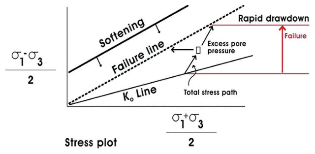
The mechanism was sudden drawdown after the flood peak: excess pore pressure remained in the bank while strength softened, so the failure line fell as the load rose.
A practical lesson came from the council’s lead engineer. Traffic was stopped on the six-lane road along the top of the banks to unload the crest, and the emergency crews then parked their vehicles on the empty road, replacing moving traffic with static load.
For railroad work: the post-flood period is when river-bank and embankment-toe slides develop, so inspections should continue through the recession, not stop at the peak. If a crest is being unloaded, the instruction has to cover equipment staging, and train restrictions should not be replaced with parked work equipment.
Source: Look, B. G. (2023). Earthworks: Theory to Practice – Design and Construction. CRC Press/Balkema. Case study §9.7, pp. 302–304. Summarized and paraphrased; figures reproduced for internal reference. Full reference under Supplemental Sources.
Authors: Daniel P. Colwell and Mario Ruel. This chapter was written and compiled by Daniel P. Colwell and Mario Ruel for Railway Ground Hazard Risk Management.
Technical content is drawn from the published sources below, and credit for that material belongs to their authors and publishers. Tables, equations and figures taken from a specific source are also cited where they appear.
File locations for these documents are listed under Supplemental Sources — LEVI Library.
Material in the green “Supplemental reference” boxes throughout this chapter was added from the following documents in the LEVI geotechnical library. Text is summarized or paraphrased; tables are reproduced with their original source noted; figures are reproduced from the cited document for internal reference use. Consult the original document before relying on a value for design. Blocks marked “After Selig & Waters (1994)” summarize item S9 for railroad clients; tables are condensed from the book and its figures are not reproduced. The Case Studies section summarizes case studies from item S10 by Burt G. Look; its figures are reproduced from the book for internal reference use, and the closing “For railroad work” note in each case study is added by the authors of this manual. Blocks tagged “Project management” summarize methods, examples and figures from the project-management, estimating and construction-management books listed here, applied to railroad work; the closing “For railroad work” note in each block is added by the authors of this manual.